“A 3D canvas on which the artist can draw using trilaterated coordinates from ultrasonic delays.”
Project Soundbyte
For our final project in ECE 4760, we designed and implemented a three-dimensional paint program consisting of hardware, a microcontroller, and a PC running MATLAB. All three modules strongly interacted to allow the artist to wave a pen around in space and see their movements translated in real time to various projections on the computer.
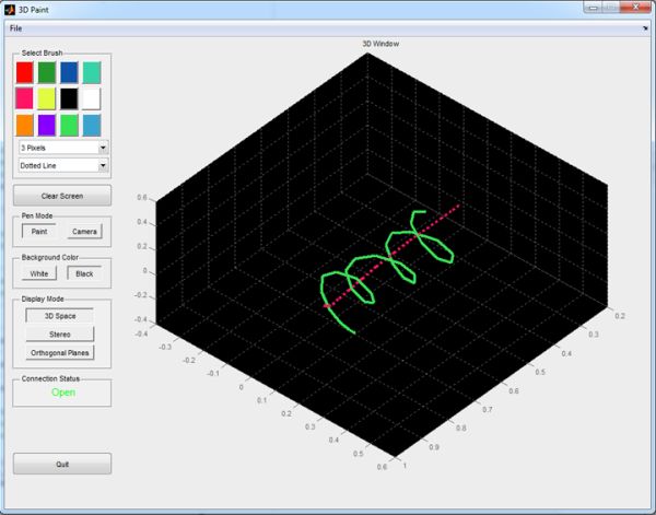
An ATmega644 microcontroller calculates the time delay from the pen to three known points and communicates these values continuously to a PC running MATLAB via a serial port. MATLAB then translates the delay information to real xyz-coordinates and displays the data in various forms on a fully functional GUI. The artist can additionally use the pen as a camera to look around the design space.
We wanted to create this system as a facilitator of creativity. Because of the strong relationship between the artist and the medium, we hoped that a new take on the canvas would instigate new creative processes. This idea encouraged us to create a device as simple as possible so that as little technological bias would be injected as possible.
High Level Design top
Overview
When contemplating ideas for final projects, we decided to rigidly follow a set of specific stipulations. First, we wanted to implement something new that would be a genuine joy to use and build rather than implement something just because it was technologically difficult and would satisfy the requirements of the class. Because this project is often thought of as the culmination of a Cornell ECE’s undergraduate career, we wanted to build something that relied on many aspects of our education: physics, mathematics, analog and digital circuits, signal processing, microcontroller programming, peripheral communication, and high-level coding to name a few.
The original idea was to design a system for tracing out 3D objects so that someone could, for instance, take a pen and trace out a coffee mug and then build a 3D model out of it in a computer for use in animation or finite element modeling. Physical limitations quickly took effect, however. Because you would rarely have line-of-sight between receiver and transmitter due do whatever object you were tracing, you would need to communicate via radio waves. We searched for possible ways to accurately measure distances based on this, including via the amount of power received between an RFID tag and reader, but to our knowledge distances have only been accurate with this method to around 10 cm, which is far outside acceptable bounds for the application. Our research yielded no way to proceed with RF using relatively simple hardware, so the natural progression of this idea was to remove the object being traced.
By removing the object, it was now possible to maintain line-of-sight between Rx/Tx pairs at all times. The idea was now simply a 3D paint program that had a plausible implementation through high frequency sound and the known propagation delay of acoustic waves to trilaterate distances.
With this core idea in place, ideas bloomed for how to make the system fun to use. By interfacing with MATLAB we could display the drawing in high quality plots that were perfect for exporting. Further, MATLAB supports full GUI design, so we could make a nice interface for the artist to select various brush sizes, colors, and styles. Bruce Land also suggested we have a stereoscopic representation of the drawing. To make the drawing process more fluid, we decided to have the program operate in a ‘paint’ mode to draw or in a ‘camera’ mode in which the artist could use the pen as a virtual camera to look around their drawing.
Mathematical Background
The foundation for the device relies on the fact that the speed of sound is constant in a given medium. Under everyday conditions, the speed of sound in air is 340.29 m/s. This means that we have a bijective mapping between time and distance for sound propagation. By emitting a sound pulse and recording the time delay between emission and detection, we calculated a displacement via the following equation:

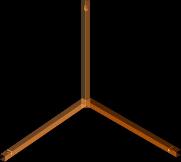
One delay measurement will give you a position in one dimension along the line-of-sight of the transmitter and receiver, yet in three dimensions all a single delay value will tell you is that the emitter was somewhere on the surface of a sphere centered at the receiver and with a radius equal to the time delay multiplied by the speed of sound. To determine a true xyz-coordinate, we needed to get more delay measurements. Positioning another receiver uniquely will give you two spheres of possible locations centered around each receiver, and the two sphere’s intersection (generally a two-dimensional circle) will give you all the possible locations that satisfy both delay measurements. Adding yet another unique receiver will further stipulate the position of the pen, but this time exactly. The resulting coordinate system and placement of the three receivers can be seen below.
We now have three equations (spheres located around each receiver) and three unknowns (where l is the displacement of each receiver along a given axis), thus a single unique position for the pen can be determined.
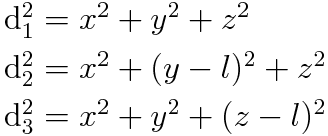 Three sphere equations
Solving this system of equations can be tricky, but noticing that some equations can be subtracted from one another greatly simplifies calculation. The z and y coordinates can be calculated directly from the delay measurements, and then using these values x can be solved for. You end up with the following:
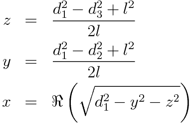 Trilateration equations for our setup
Note that we are taking the real part of the square root in the x calculation. If our delay measurements were mathematically perfect this would be an irrelevant calculation because the square root argument would never be negative. However, because the data is imperfect it is certainly possible for the square root to produce imaginary results. Taking the real part is a very good approximation given the imperfect data, however. These equations allow us to perform what is called a trilateration.
Logical Structure
There were three primary components involved with the system: the microcontroller, the hardware, and the PC running MATLAB.
The microcontroller’s primary function was to facilitate the rapid acquisition of time delays between the transmitter and three receivers. This job was tasked to a microcontroller because of its inherent ability to interface with analog hardware and communicate with higher-level machines like a PC. The microcontroller coordinated the emission of a sound pulse according to many timing specifications. For instance, it could not emit too fast or the receivers would become confused as to which received pulse corresponded to which emitted pulse. Additionally, some receivers might not have received a pulse if the pen was directed away at too great an angle so it needed to be prepared to handle measurement timeouts. The microcontroller was responsible for keeping all pulses and receptions locked in step to ensure quality data. Originally the microcontroller was not tasked with any signal processing requirements, yet this job was also later assigned to it to improve responsiveness. The microcontroller was also to follow a protocol to transfer data up to MATLAB. When MATLAB requested data, the microcontroller was to respond via UART serial communication with a packet containing information relating to the pen’s status (button pushed or not) and the three delay values.
The hardware was further broken up into two components: emission and detection. The microcontroller produced a 40 kHz square wave suitable for the ultrasonic Tx/Rx pairs we used. However, the microcontroller could not generate signals sufficient enough to properly drive the transmitter (it could handle 30 V peak-to-peak values but the ATmega644 was limited to 5 V peak-to-peak output). Thus, the 40 kHz signal required significant gain to maximize the strength of acoustic pressure waves and therefore maximize directionality (wider is better), possible distance from receivers, and signal-to-noise. Further, hardware was responsible for providing the artist with an easy way to specify whether or not they wanted to be painting a stroke at a given moment. This was accomplished via a button mounted on the pen (so it was collocated with the transmitter). On the reception side the hardware had to gain the received voltages such that they were interpretable by the microcontroller.
MATLAB was where the bulk of the artist interaction was centralized. It was to produce a fully functional GUI so that the artist could change various parameters about the paintbrush (i.e. color, etc.) and receive visual feedback as to what they were drawing. MATLAB was to provide a variety of options for how the feedback was displayed (3D plot, 2D orthogonal projections, etc.). MATLAB needed to request data from the microcontroller and parse it into xyz-coordinates via the trilateration equations above. It also needed to parse the state of the push button to determine whether or not to draw a stroke. When the artist was not drawing, MATLAB was still to display a cursor of the current location of the pen. When the program was in ‘camera’ mode MATLAB was to interpret the pen position as the location of a camera so that the artist could look around their drawing. Further, MATLAB had minimal signal processing requirements to further smooth the data. Finally, MATLAB needed the ability to export the drawing as a jpeg.
Hardware and Software Trade-offs
Our design philosophy was to simplify the device as much as possible so as not to impede upon the artist’s work-flow. To this end, we designed the system with minimal hardware UI and instead concentrated the UI in software. Accordingly, we implemented the pen with a single critical button to indicate drawing or not drawing. The button was located toward the front of the pen so that the artist could hold it and press it only when they wanted to make a stroke. Obviously, having software UI for this function would be comparatively cumbersome. For the rest of the UI, we could have used hardware buttons or toggle switches but software seemed a more appropriate choice. We wanted to limit the physical footprint of the device, and running a bunch of wires to and from physical buttons seemed unnecessarily complex for something like selecting the brush color. Putting these sorts of options in hardware also meant that the microcontroller was responsible for capturing and relaying button states up to MATLAB. This was inefficient a) because the microcontroller did not need to know the button states and b) because it would waste cycles and time to capture and transmit them (UART communication is very slow, so data should not be sent unless it is absolutely necessary). Further, implementing these options in software made the program much more extensible: new features could simply be added in code without any new hardware development.
The rest of the hardware/software breakdown was predicated entirely by the limitations of hardware and software and thus didn’t require a strategic breakdown.
The MATLAB/ATmega644 break down was a harder line to walk. Initially we only wanted the 644 to record delay information and send it up so that it could run as fast as possible. However, we quickly discovered that one of our greatest bottlenecks was how quickly MATLAB could process a given delay packet, put it out on all plots, and update the cursor position. So, it happened that the ATmega644 could produce delay information much faster than MATLAB could read it. Because MATLAB was originally doing the DSP operations, this meant a fairly substantial delay (~500 msec) from physical movement to display on the GUI because of the time it took for new data to fill up the sliding window buffers used for processing. To fix this, we off-loaded the signal processing to the microcontroller, which meant that the MATLAB code would instead receive already filtered data, and the responsiveness of our system increased tremendously.
Standards
Given the relatively simple hardware involved in this project, few standards were used in implementing communication between the PC and the peripheral device (MCU). Serial communication between the MCU and the PC made use of the MCU’s onboard universal synchronous/asynchronous receiver/transmitter (USART) peripheral unit and took place via the STK500’s Serial port and PC’s USB port. As it was only used asynchronously, it may be referred to as a UART. This UART was used in conjunction with the RS-232 communication standard.
Intellectual Property (Patents, Copyrights, and Trademarks)
We chose to name our completed product 3D Paint, which may potentially infringe on the Paint trademark held by the Microsoft Corporation for its own graphics painting program. If this becomes an issue, we can opt to change the name of our product.
We do not believe that the technology infringes on any existing patents. In Relevant Patents, we have linked a number of patents relating to ultrasonic three-dimensional positioning systems. There is also another student project for ECE 4760 from Spring 2009 (UltraMouse 3D by Karl Gluck and David DeTomaso), which makes similar use of ultrasonic sensors for three-dimensional positioning, but only accurately records two-dimensional coordinates. However, as our design uses different methods to detect pulses and filter data, we do not believe that we have violated any of them.
Software Design & Implementation top
The software was implemented across two platforms: the ATmega644 and MATLAB.
Microcontroller
The microcontroller code was written to be as straightforward as possible. It operated within a while(1) loop after some basic initialization procedures. Initialization procedures included setting up UART communication (we used a baud rate of 38500 to speed up communication), configuring i/o pins, initializing timers, setting up interrupts and initializing variables.
The code required the use of all three timers provided by the ATmega644. We used timer0 to establish a .5 msec time base from which we could dispatch various actions (like initiate a new pulse train or signal a timeout). Timer1 was used as a means to calculate the delay in cycles that it took for a pulse to be detected. Because we wanted to time as accurately as possible, timer1 was counting at the full clock speed (16 MHz) of the MCU. This corresponded to a range resolution of roughly 21 μm, which was more than acceptable for the purposes of the system. Timer2 was utilized to generate the 40 kHz square wave required by the ultrasonic Tx/Rx pair.
Five interrupts had to be written for proper operation of the code. First was the timer1 overflow interrupt. This interrupt was triggered every time timer1 (an 8 bit counter) overflowed. Because 8 bits was not nearly enough space to represent a typical delay time in cycles (they were generally on the order of 10,000 cycles), we simply had the overflow interrupt increment a variable by 256 every function call so that we could keep track of the true cycle count. The second interrupt ran whenever we received a new character on the serial port. This was used to indicate to the program that MATLAB had sent a command and that the 644 would need to respond. The other three interrupts were hardware interrupts on int0 (pin D.2), int1 (pin D.3), and int2 (pin B.2). Each ultrasonic Rx was wired up to a given pin after gain, so the interrupt would fire when the pulse was received. This allowed us to stop the timer on the delay count. There is an alternative way to do this, and was implemented in the ‘3D Ultrasonic Mouse’ project for ECE 4760 by Karl Gluck and David DeTomaso. They had an interrupt fire periodically at 160 kHz and poll the receivers for an acquired pulse. We felt better about the interrupt-driven scheme because of the innate aperiodic nature of the pulses coming in. Polling at 160 kHz automatically limits your resolution to 2 mm, whereas our scheme imposes no set limitation on resolution. Obviously, the drawback of the interrupt method is interrupt collisions, or when two or three receivers receive a pulse all at the same time. We tested this, and found that for this worst case scenario it took roughly 100 cycles to get in and out of a given interrupt, implying a maximum error of 200 cycles if they all interrupted at exactly the same time. While this maps to an error of 4 mm, it is only for an extremely small subset of the drawing space where the pen is equidistant to all receivers. For the overwhelming majority of the space, however, we saw a negligible error using the interrupt method.
After initialization the code entered a while(1) loop and constantly checked a number of conditions. First it updated the state of the pen button, which was fully debounced, every 20 msec. The button debounce code was written by Bruce Land and was provided on the 4760 course webpage. The button debounce code had a variable containing the current state of the button (i.e. pushed or not pushed). This variable was what was sent to MATLAB to indicate whether or not the artist was drawing.
Next the code checked whether or not it was time to emit a new pulse. We set the inter-pulse period (IPP) to 20 msec for this lab to ensure that any reflections from previous pulses would have plenty of time to die out before we began a new measurement. This corresponded to a distance of roughly 6.8 meters, which was plenty in practice. If it was time to emit a new pulse train, we reinitialized all timing variables and also rearmed the interrupts. By rearming, we mean that each interrupt would only record a value if it were armed. This prevented a lot of misfiring and ensured a given receiver was not constantly retriggered while waiting for one of the others to trigger. We also only emitted a pulse for .5 msec. This was all that was necessary to properly trigger the receivers, and going any longer than this would potentially confuse the receivers when operating in steady state. Limiting the length of the pulse helped to keep the environment quiet for each pulse. The loop also checked for a potential timeout. If all three receivers had not been triggered within 7.5 msec (a distance of 2.5 m) then the system would reinitialize everything, throw out the bad data, and emit another pulse. This was to guarantee that any data that was captured came from one unique pulse.
The loop also checked for whether or not all three receivers had triggered. If they had, it entered them into the signal-processing buffer. We converged on a two-stage processing scheme for this project. First we performed a sliding window median filter. The median filter was a crucial first step because it was possible for there to be very large outliers compared to the true delay. These were most often caused by pulses that reflected and triggered a receiver after the system had already reinitialized and sent out a new pulse. Median filters were preferable to some type of low pass average filter because the large outliers would still put huge skews in the data if averaged, but be completely removed if mediated. There were a few implementation challenges to getting the median filter working. First, we wanted to create a buffer that would take the median of the x most recent delay samples. To do this, we created an index to an array that would cyclically drop samples into the buffer. We first placed the sample at index 0, then index 1, and so on all the way up to index x-1, where it would modularly roll back to 0. This made it so that we didn’t need to move any values around in the array when a new sample came in. Next, we needed to sort the data (as this is typically the most efficient way to find a median). The C standard library provides a function qsort that accomplished this for us so long as we provided a compare function for whatever data type we were sorting. Because we needed to maintain the order of the buffer for proper windowing, we had to copy the data to a temporary array, sort it, and then extract the median by simply looking at the middle array index. In steady state this produced a new median filtered delay value every time we captured a new sample. We found a median length of five produced excellent stability and responsiveness.
Parts List:
| Electronics | STK 500 | P | ECE 4760 Lab | $15.00 | 1 | $15.00 |
| Mega644 | P | ECE 4760 Lab | $6.00 | 1 | $6.00 | |
| 9V Power Supply | P | ECE 4760 Lab | $5.00 | 1 | $5.00 | |
| Ultrasonic Tx/Rx Pair (Jameco Valuepro 40T/R-12B) | P | Jameco (Part No.: 139492) | $7.95 | 2 | $15.90 | |
| 1.5A Dual Mosfet Driver (Microchip TC4428AEPA) | P | Jameco (Part No.: 1292826) | $1.09 | 1 | $1.09 | |
| Instrumentation Amplifiers (Texas Instruments INA129) | S | Texas Instruments Inc. | $0.00 | 3 | $0.00 | |
| Connections | Small Solder Board (2 inch) | P | ECE 4760 Lab | $1.00 | 1 | $1.00 |
| 8 pin DIP Socket | P | ECE 4760 Lab | $0.50 | 4 | $2.00 | |
| SIP Socket | P | ECE 4760 Lab | $0.05 | 13 | $0.65 | |
| SIP Plug | P | ECE 4760 Lab | $0.05 | 3 | $0.15 | |
| Header Socket | P | ECE 4760 Lab | $0.05 | 9 | $0.45 | |
| Wire | F | ECE 4760 Lab | $0.00 | N.A. | $0.00 | |
| Button | F | ECE 4760 Lab (Scrap) | $0.00 | 1 | $0.00 | |
| Resistors and Capacitors | Through-Hole 10Ω Resistor | F | Already owned | $0.00 | 3 | $0.00 |
| Through Hole 0.1µF Capacitor | F | Already owned | $0.00 | 3 | $0.00 | |
| Physical Structures | Pen Casing | F | Already owned | $0.00 | 1 | $0.00 |
| 3 foot wooden plank | F | Already owned | $0.00 | 3 | $0.00 | |
| Screw | F | Already owned | $0.00 | 2 | $0.00 | |
| Nut | F | Already owned | $0.00 | 2 | $0.00 | |
| Washer | F | Already owned | $0.00 | 2 | $0.00 | |
| Total | $47.24 |
For more detail: 3D Paint Using Atmega644