Summary of Brain-Computer Interface Using Atmega644
Summary: A low-cost brain-computer interface was built using an Atmega644 AVR to record EEG via saline silver-plated electrodes, amplify and filter the microvolt signals, digitize them with the MCU ADC, and send ASCII ADC values over an opto-isolated USB UART to a PC. PC software in MATLAB and C/OpenGL performs FFT, FIR filtering, SVM classification, P300 experiments, neurofeedback, and controls a Pong game via alpha and mu rhythm modulation. Hardware includes a two-stage amplifier (AD620 + 3140 op amp), battery-powered isolation, and an EEG electrode cap following the 10-20 system.
Parts used in the Brain-Computer Interface Using Atmega644:
- SparkFun COM-00102 SPDT Mini Power Switch
- Green LED
- 1 MΩ Resistors
- 1 kΩ Resistors
- 100 Ω Resistor
- Jumper Wire
- Digi-Key BC4AAW-ND Battery Holder 4-AA Cells
- AA Batteries (Panasonic Alkaline Plus)
- Digi-Key 160-1791-ND Fairchild Semiconductor 6N137 Opto-Isolator
- 0.01 μF Capacitor
- 220 Ω Resistor
- 1.1 kΩ Resistor
- DIP Socket
- Digi-Key AD620ANZ-ND AD620 Instrumentation Amplifier
- Digi-Key CA3140EZ-ND CA3140 Operational Amplifier (two units)
- Digi-Key 3386F-105LF-ND 1 MΩ Trim Potentiometer
- 0.0068 μF Capacitor
- 1 μF Capacitor
- 0.22 μF Capacitors
- 2.2 kΩ Resistors
- 10 kΩ Resistor
- 15 kΩ Resistors
- Mega644 microcontroller
- FTDI USB Comms Board
- Target Board
- Target Board Socket
- Female Wire Headers
- Female Wire Sockets
- White Board
- Solder Board (6 inch)
- Ten Pack Silver Plated Electrodes (Contec Medical Systems)
- Baseball Cap (for electrode helmet)
Introduction
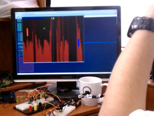
Our goal was to build a brain-computer interface using an AVR microcontroller. We decided that the least invasive way of measuring brain waves would be using electroencephalography (EEG) to record microvolt-range potential differences across locations on the user’s scalp. In order to accomplish this, we constructed a two-stage amplification and filtering circuit. Moreover, we used the built-in ADC functionality of the microcontroller to digitize the signal. Passive silver-plated electrodes soaked in a saline solution are placed on the user’s head and connected to the amplifier board. The opto-isolated UART sends the ADC digital values over USB to a PC connected to the microcontroller. The PC runs software written in MATLAB and C to perform FFT and run machine learning algorithms (SVM) on the resultant signal. From there, we were able to control our own OpenGL implementation of the classic PC game Pong using our mind’s brain waves. We also wrote software to record our sleep and store the EEG signal inside a data file.
High-Level Design
Rational and Inspiration for Project Idea
Our project idea was inspired by Charles’s severe obstructive sleep apnea (OSA) disorder. In order to diagnose sleep apnea, a clinical sleep study is performed where the patient is attached to EEG electrodes, along with SpO2, EMG, and respiration sensors. The patient’s sleeping patterns are recorded overnight, and apneas (periods of sleep without breathing) can be identified within the collected data. This process is costly and requires an overnight stay at a hospital or sleep lab. Moreover, the patient often is denied access to their own data since a licensed sleep specialist interprets it for them. Our goal was to build a low-cost alternative that would allow users to take their health in their own hands by diagnosing and attempting to treat their own sleep disorders. Moreover, our project has diverse applications in the areas of neurofeedback (aiding meditation and treatment of ADHD disorder), along with brain-computer interfaces (allowing the disabled to control wheelchairs and spell words on a computer screen using their thoughts).
Background Math
Support Vector Machines
The machine learning algorithm we used was a support vector machine (SVM), which is a classifier that operates in a higher dimensional space and attempts to label the given vectors using a dividing hyperplane. The supervised learning method takes a set of training data and constructs a model that is able to label unknown test data. A brief explanation of the mathematics behind SVMs follows. During training, the SVM is given a set of instance-label pairs of the form {(xi⃗ ,yi):i=1,…,l} where the instances are n-dimensional vectors such that xi⃗ ∈Rn. The n dimensions represent n separate “features.” In addition, the labels are in the form y∈{1,−1}, where 1 and -1 designate target and non-target instances respectively. To “train” the support vector machine to recognize unknown input vectors, the following minimization problem is solved:
subject to:
Source: http://www.csie.ntu.edu.tw/~cjlin/papers/guide/guide.pdf
Note that ϕ is a function that maps the training vectors x⃗ i into a higher-dimensional space, while C>0 and ξi act as error terms (so-called “slack variables”). Moreover, K is the kernel function which is defined as K(ϕ(xi)Tϕ(xj)). For our purposes, we used a radial basis function (RBF) kernel which has a K function of K(xi,xj)=exp(−γ||xi−xj||2) where γ>0 represents a user-tunable parameter.
DFT
The discrete Fourier transform (DFT) transforms a sequence of N complex numbers (an N-point signal) in the time-domain into another N-sequence in frequency domain via the following formula:
The Fourier transform is denoted by F, where X=F(x). Source: http://en.wikipedia.org/wiki/Discrete_Fourier_transform
An algorithm, the Fast Fourier Transform (FFT) by Cooley and Tukey, exists to perform DFT in O(nlogn) computational complexity as opposed to O(n2). We take advantage of this speed-up to perform DFTs in real-time on the input signals.
Filters
In order to filter the brain wave data in MATLAB, we use a finite impulse response (FIR) filter which operates on the last N+1 samples received from the ADC. In signal processing, the output y of a linear time-invariant (LTI) system is obtained through convolution of the input signal x with its impulse response h. This h function “characterizes” the LTI system. The filter equation in terms of the output sequence y[n] and the input sequence x[n] is:
Note that only N coefficients are used for this filter (hence, “finite” impulse response). If we let N→∞, then the filter becomes an infinite impulse response (IIR) filter. Source: http://en.wikipedia.org/wiki/FIR_filter
EEG Signal Analysis
The EEG signal itself has several components separated by frequency. Delta waves are characteristic of deep sleep and are high amplitude waves in the frequency range 0≤f≤4 Hz. Theta waves occur within the 4-8 Hz frequency band during meditation, idling, or drowsiness. Alpha waves have frequency range 8-14 Hz and take place while relaxing or reflecting. Another way to boost alpha waves is to close the eyes. Beta waves reside in the 13-30 Hz frequency band and are characteristic of the user being alert or active. They become present while the user is concentrating. Gamma waves in the 30-100 Hz range occur during sensory processing of sound and sight. Lastly, mu waves occur in the 8-13 Hz frequency range while motor neurons are at rest. Mu suppression takes place when the user imagines moving or actually moves parts of their body. An example diagram of the EEG signal types follows:
EEG signals also contain event-related potentials (ERPs). An example is the P300 signal, which occurs when the user recognizes an item in a sequence of randomly presented events occurring with a Bernoulli distribution. It is emitted with a latency of around 300-600 ms and shows up as a deflection in the EEG signal:
Logical Structure
The overall structure of the project consists of an amplifier pipeline consisting of a differential instrumentation amplifier (where common-mode noise is measured using a right-leg driver attached to the patient’s mastoid or ear lobe), along with an operational amplifier and some filters (to remove DC offsets, 60 Hz power-line noise, and other artifacts). From there, the signal passes to the microcontroller, where it is digitized via an ADC. Next, it is send over an isolated USB UART connection to a PC via an FTDI chip. The PC then performs signal processing and is able to output the results to the user, creating a neurofeedback loop which allows the user to control the PC using their brain waves. A functional block diagram of the overall structure follows:
Hardware/Software Trade-offs
Performing FFT in hardware using a floating-point unit (FPU) or a field programmable gate array (FPGA) would have allowed us to realize a considerable speed-up; however, our budget was only limited to $75, so this was not an option. Another trade-off we encountered was the use of MATLAB versus C. MATLAB is an interpretted language whose strength lies in performing vectorized matrix and linear algebra operations. It is very fast when performing these operations, but it is an interpreted language that does not run as native code. This speed penalty affected us when we attempted to collect data in real-time from the serial port at 57600 baud. To combat this speed penalty, I wrote a much faster OpenGL serial plotting application in C that runs at 200-400 frames per second on my machine (well above the ADC sample rate of 200 Hz) and is able to perform FFTs in real-time as the data comes in. Furthermore, yet another trade-off was the decision to use the PC to output the EEG waveforms rather than a built-in graphical LCD in hardware. Once again, budget constraints limited us, along with power usage since for safety reasons, our device uses four AA batteries instead of a mains AC power supply.
Relationship of Your Design to Available Standards
There exists a Modular EEG serial packet data format that is typically used to transmit EEG data over serial; however, we used ASCII terminal output (16-bit integer values in ASCII separated by line breaks) for simplicity, ease of debugging, and compatibility with MATLAB. Moreover, serial communications followed the RS232/USB standards. Another consideration was the IEC601 standard. IEC601 is a medical safety standard for medical devices that ensures that they are safe for patient use. Unfortunately, testing for IEC601 compliance was very much out-of-budget. Nevertheless, we discuss the many safety considerations that we absolutely adhered by in the Safety subsection (under Results) of this report.
Hardware Design
Amplifier Board Design
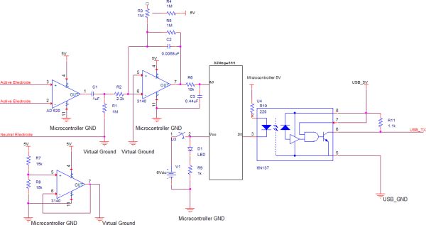
We built an analog amplification circuit with a total gain of 1,500 based on the design by Chip Epstein at https://sites.google.com/site/chipstein/home-page/eeg-with-an-arduino with modified gain and filter stages. The first stage uses an AD620 instrumentation amplifier for differential common mode signal rejection to reduce noise. The gain of the AD620 is approximately 23. A voltage divider and a 3140 opamp buffer provide a 2.5 V virtual ground for the instrumentation amplifier. After passing through the instrumentation amplifier, the signal is filtered using an RC high pass filter with fc=0.13 Hz (we modified the original design to allow the P300 ERP to reside within the pass-band of the filter).
Next, the signal undergoes a second-stage amplification. The gain of a 3140 opamp is set to approximately 65. The output signal is then filtered using an RC low-pass filter with a cut-off frequency of approximately 48 Hz. This frequency was chosen to preserve the low-frequency content of the EEG signal, while removing 50-60 Hz power line noise from the signal. We ordered parts from Digi-Key and samples from Analog Devices, Texas Instruments, and Maxim Semiconductor. We also sampled silver-plated passive EEG electrodes. From there, we were able to amplify a 125 μVVpp, 10 Hz square wave calibration signal to well within the ADC reference voltage range (0-1.1 V) and plot it on a PC in real-time. We constructed this prototype circuit on a breadboard. A schematic diagram of the amplifier board follows:
Microcontroller Board Design
The microcontroller board contains a voltage divider that outputs a 125 μVVpp, 10 Hz square wave calibration signal from Pin D.3 of the microcontroller. Moreover, it contains a +6V DC battery-power supply that provides DC power to the microcontroller and the amplifiers. A schematic diagram of the microcontroller board follows:
Opto-Isolated UART over USB Design
We constructed an isolated +6 VDC power supply using 4 AA batteries and connected it the microcontroller using the PCB target board. We cut the ground trace connecting the microcontroller ground to the USB ground using a dremel tool. An illustration of the cut that we performed follows:
We used a Fairchild Semiconductor 6N137 optoisolator to isolate the USB power from the microcontroller power. The line of isolation is between the microcontroller UART RX and TX pins (Pin D.0 and Pin D.1) and the FTDI chip’s RX and TX pins. A schematic diagram of the isolation circuit follows:
Electrode Cap Design
We constructed an EEG helmet consisting of an old baseball cap modified to contain EEG electrodes. We followed the International 10-20 System of Electrode Placement by including electrodes at the designated locations on the scalp: Occipital lobe (O), Central lobe (Fz, Pz, C3, C4, Cz), and Frontal lobe (Fp1, Fp2, G). A diagram of the 10-20 system of electrode placement follows:
Software Design
MATLAB Serial Code
The primary function of the MATLAB serial code is to acquire digital EEG signal data from the microcontroller over the serial port. We wrote some code to plot the signal onto the screen and to perform rudimentary signal processing tasks (FFT and filtering). The MATLAB code consists of three files: plot_samples.m, plot_samples_rt.m, and serial_test.m
The serial_test.m script opens the serial port and displays an almost real-time plot of the serial data. It parses the serial data in a while loop via fscanf and str2num. Additionally, it updates the plot window contents using MATLAB’s drawnow command. The loop terminates if the user closes the plot window, causing the script to clean up the file handle and close the serial port.
The plot_samples.m script opens the serial port, and reads exactly N=200 samples of EEG data (around 2 seconds). It then closes and cleans up the serial port. Next, a 60 Hz notch filter is applied to the signal to remove powerline noise via the iirnotch and filter, and the DC offset (mean value) is subtracted from the signal. Finally, the time-domain signal is displayed in a plot window, along with the single-sided amplitude spectrum computed via MATLAB’s fft function.
The plot_samples_rt.m script performs exactly the same operations as the plot_samples.m script, except it performs them in a loop. The script operates by sampling N=200 samples repeatedly until the user closes the plot window. As an effect, the signal plot and the frequency spectrum are refreshed every 2 seconds giving psuedo real-time operation.
OpenGL Plotter
A real-time serial plotter was written in OpenGL and C++. OpenGL is a high-performance graphics library, while C++ is much faster than MATLAB since it runs as native code. The program displays the real-time wave form from the serial port, along with its FFT. We use the FFTW (Fastest FFT in the West) library for computing the FFT using fast algorithms. Moreover, extensions were later added to the plotting code allow Pong to be played using brain waves, along with a P300 ERP detector. A data logging feature was added to allow us to record our EEG data while asleep to a file. The SDL library is used to collect user input from the keyboard and output the OpenGL graphics buffer to an on-screen window.
nitialization and Event Loop
The main() function initializes the SDL library, clears the ADC buffers, initializes OpenGL, initializes SDL TTF (for True Type font rendering), opens the serial port, opens the log file, and initializes the FFTW library. From there, the program enters the main event loop, an infinite while loop which checks for and handles key presses, along with drawing the screen via OpenGL.
The Quit() function cleans up SDL, closes the serial port, de-initializes FFTW frees the font, and quits the program using the exit UNIX system call.
The resizeWindow() function changes the window size of the screen by changing the viewport dimensions and the projection matrix. For this project, we use an orthographic projection with ranges x∈[0,X_SIZE] and y∈[0,ADC_RESOLUTION]. The handleKeyPress() function intercepts key presses to quit the game (via the [ESCAPE] key) and to toggle full screen mode (using the [F1] key).
The initGL() function initializes OpenGL by setting the shading model, the clear color and depth, and the depth buffer.
Drawing Code
The drawGLScene() function is called once per frame to update the screen. It clears the screen, sets the model view matrix to the identity matrix I4, shifts the oscilloscope buffer running_buffer to the left by one, and fills the new spot in the buffer with the newest sample from the serial port. This sample is obtained by calling the readSerialValue() function in serial.cpp. This function also contains logic to perform the FFT and draw it onto the screen as well. The sample is sent to the P300 module and logged to the output file. Moreover, the power spectrum of the FFT is computed using rfftw_one() and by squaring the frequency amplitudes.
The FFT bars and the oscilloscope points are plotted using GL_LINES and GL_POINTS respectively. Moreover, lines join adjacent oscilloscope points. The frequency ranges corresponding to each brain wave classification (alpha, beta, etc.) are calculated, along with their relative powers. Moreover, BCI code is executed which will be discussed in the OpenGL Pong sub-section of this report. The pong and P300 modules are then drawn on the screen, along with status text using TTF fonts and the framebuffer is swapped. Lastly, the frame rate is calculated using SDL_GetTicks(), an SDL library function.
Serial Code
The serial code handles serial communications over USB and is located in serial.cpp. Important parameters such as the buffer size BAUD_RATE, the port name PORT_NAME, and the baud rate B57600 are stored as pre-processor directives. The openSerial() function opens the serial port and sets the baud rate to 57600 (56k). The readSerialValue() function reads and parses one 10-bit ASCII ADC value from the serial port by scanning for a new-line terminator and using sscanf (readByte() is unused). Lastly, the closeSerial() function closes the serial port device. The UNIX system calls open, read, and close are used to carry out serial I/O, along with the GNU C library’s system() function. The device file name for USB serial in UNIX is /dev/ttyUSB0.
Note that if the NULL_SERIAL pre-processor directive is set, then mock serial data is used rather than actually collecting data from the serial device. This functionality is useful for testing purposes.
Configuration
The config.h file contains pre-processor directives that can be used to configure the OpenGL plotting application during compile-time. Important parameters include the screen width and height (SCREEN_WIDTH and SCREEN_HEIGHT respectively), the screen bit depth (SCREEN_BPP), ADC_RESOLUTION the ADC resolution (the number of y-values) set to 210=1024, and the log file name LOG_FILENAME (defaulting to "eeg_log.csv").
Debugging
Useful utility functions for debugging purposes are found in debug.cpp. The FileExists() function returns a boolean indicating whether the given file exists. The OpenLog() and CloseLog() functions are useful for writing log files with time and date stamps. The log_out() function can be passed a format string which is written to the log file, along with a time stamp. The format() function takes a format string and returns the formatted result. It uses the vformat utility function to generate the format string based on the arguments passed to the function. The dump() function dumps regions of memory to the screen in a human-friendly hexadecimal format.
Font Rendering
TTF font rendering support was implemented using NeHe sample code (located in the References section of this report). The glBegin2D() and glEnd2D() functions set up an orthographic screen projection for font rendering. Meanwhile, power_of_two() is a utility function that calculates the next largest power-of-two of the given integer input (useful for computing OpenGL texture dimensions which must be powers of two). The SDL_GL_LoadTexture() function converts an SDL_Surface structure in memory to an OpenGL texture object. This is useful because the SDL_TTF library only returns an SDL_Surface, but we are rendering the fonts using OpenGL. The InitFont() and FreeFont() functions use the SDL_TTF library functions to load and free fonts respectively. Lastly, glPrint() acts like an OpenGL implementation of printf by printing strings to the screen using TTF font textures in SDL_TTF.
OpenGL Pong
The Pong game logic and drawing code is located in the pong.cpp source file. Moreover, a set of constant “glyphs” is located in the glyphs.h header file. These glyphs are 2D arrays of boolean values corresponding to pixel on and pixel off for each scoreboard number that is displayed on the screen. The blocky font used for each glyph lends a retro syling to the game (which suits the Pong aesthetics much more than the TTF font renderer would).
Pong Game Logic
The game logic defines several variables including the paddle width and height (stored in PADDLE_WIDTH and PADDLE_HEIGHT respectively), the positions of both paddles, the x and y positions and velocities of the ball (ballposx, ballposy, ballvelx, ballvely). The sprite[] array includes a boolean bitmap storing the ball sprite.
The updateball() function performances rudimentary numerical integration to get the new ball position by addition. Bounds checks is performed and the ball velocity is negated to reflect the ball direction if the ball collides with the screen edges. Collision detection is performed with both paddles for all four sides also using bounds checking. Moreover, the ball’s velocity is reflected and its speed is increased slightly by the constant value stored in vel_threshold upon colliding. Lastly, if the ball collides with the left or right side of the screen, the appropriate player’s score variable (score1 or score2) is incremented depending on which side the ball collides on. The ResetVelocity() function is invoked to reset the ball’s speed back to the initial speed.
The pongInit() function determines a random direction of the pong ball for the initial “face off” by calling a utility function randomNum() which generates a random integer in the set 0,1. The pongHandleKeyDown and pongHandleKeyUp update the game state based on keyboard presses and depresses. The [UP] key moves the right paddle up, and the [DOWN] key moves the right paddle down. The left paddle is controlled by the user’s brain waves. The updatepaddle1() and updatepaddle2() functions perform numerical integration using addition to update the paddle y velocities (paddle1yvel and paddle2yvel respectively).
Pong Game Drawing Code
The pongUpdateAndRender() function is invoked from the OpenGL plotter drawing code. It invokes all of the updating functions (updateball(), updatepaddle1(), updatepaddle2()) and all of the drawing functions (drawsprite(), drawpaddlesprite(), drawscore(), and drawline()). The drawscore() function draws both score glyphs onto the screen at the proper positions by invoking drawglyph(). The drawglyph() function takes an integer number, an x and y position, and an (r,g,b) floating point color value. It uses GL_POINTS to draw each pixel of the glyph onto the screen. The drawsprite() function takes an (x,y) position and an (r,g,b) color and draws the ball sprite at that location. The drawline() function draws a striped line with spacing defined by LINE_SPACING across the center of the screen depicting the center of the field. Finally, the drawpaddlesprite() function takes an (x,y) position and an (r,g,b) color and draws the rectangular paddle sprite using GL_POINTS.
Pong Brain Wave Control and Brain-Computer Interface (BCI) Code
The most important part of the Pong software is the code snippet in main.cpp that updates the left paddle velocity based on the user’s brain waves. We provide two modes of control. The first, alpha rhythm (8-13 Hz) modulation, provides proportional control based on the user’s alpha waves. The EEG electrodes are placed on the user’s forehead (near frontal lobes) during alpha rhythm measurement. The user concentrates to move the paddle down and relaxes to move the paddle up.
The other method of control is based on mu rhythm (8-13 Hz) suppression. The user imagines moving their feet up and down (or actually moves them) to move the paddle, and if mu suppression reaches a threshold, then the paddle moves down; otherwise, it moves up. The user places the electrodes on the top of the scalp near the sensorimotor cortex (10-20 locations C3 and C4) during mu suppression measurement. Although both methods worked equally well, we found during user testing that users preferred the alpha modulation control method over the mu rhythm suppression method.
Alpha Rhythm Modulation
The alpha rhythm modulation control is determined by two boundary variables ALPHA_MIN and ALPHA_MAX. The paddle’s y position posy is proportional to the alpha rhythm’s relative power spectrum’s value within this range [ALPHA_MIN,ALPHA_MAX]. From our testing, we found that values of 0.01 and 0.04 worked best for ALPHA_MIN and ALPHA_MAX respectively. Users were able to control the paddle position quite accurately after some practice.
Mu Rhythm Suppression
The mu rhythm supression control is determined by one threshold value MU_THRESHOLD. The paddle’s y velocity paddle1yvel is set to a value of 0.1 if the mu rhythm’s relative power spectrum is below MU_THRESHOLD (indicating mu suppression, or movement visualization in the user). The paddle1yvel is set to −0.1 if the mu rhythm’s relative power spectrum exceeds or matches MU_THRESHOLD. Users were also able to use this method of control albeit less successfully due to the weaker signal received from placing the saline electrodes on the user’s hair rather than their forehead. Nevertheless, mu rhythm suppression was also a viable control scheme.
Neurofeedback and Cursor Control
The alpha modulatiom and mu supression control schemes have diverse applications beyond simply playing the game Pong in brain-computer interfaces. Wheelchair and cursor control (both 1D and 2D) have been accomplished by mu rhythm suppression. In one instance, users controlled a cursor in 2D by imagining clenching either their left hand, their right hand, or moving their feet. This control scheme requires three channels measure three locations of the sensorimotor cortex near the top of the scalp: user’s left side (C3), center (Cz), and user’s right side (C4). Even though we had one channel, we could easily extend this to support 2D cursor control, along with detecting eye blinking artifacts for “clicking” the mouse. One could imagine applying this technology to allow users with special needs to control computer mouse movement.
The other application is in the field of neurofeedback. Neurofeedback creates a feedback loop for users attempting to meditate or treat ADHD disorder. The user visually sees or audibly hears the power of their alpha waves and is able to manipulate their alpha intensity. This neurofeedback has applications in the military and aircraft control as well, as users can be trained to focus and are alerted if they lose concentration. The Pong game can be viewed as a neurofeedback device since the user’s concentration level is visually depicted on the screen as the position of the left paddle. Thus, the Brain-Computer Interface component of this project has diverse applications that go far beyond playing a simple computer game with one’s brain waves.
P300 Detector
The P300 detection code was an attempt to detect which color a user is thinking of from a discrete set of randomly flashed colors displayed on the screen. The software used machine learning algorithms for support vector machines (SVMs) provided by the libSVM C library. This attempt was not successful. In a training set of 50 trials, we were unable to obtain classification accuracy beyond 64%. Nonetheless, we document our code here and provide some suggestions for improvements and future work.
The P300 code uses a finite state machine (FSM) to display colors randomly on the screen in either a training mode or a testing mode. The colors are chosen randomly from the set {red, green, blue, yellow, purple}, and after each color in the set has been displayed exactly once, a trial is considered to have been completed. Five trials are performed during both testing and training, and the recorded brain waves are averaged. The idea is to attempt to classify one-second sets of brain data as either containing a P300 potential (target) or not (non-target) using the SVM. The target set corresponds with the color that the user is thinking of. While the colors are flashed on the computer screen, the user is instructed to count the number of times the target appears.
Code Structure
The code contains pre-processor definitions (TRAINING_DATA_FILENAME and TESTING_DATA_FILENAME) for the data file names, along with configuration variables for the number of colors NUM_COLORS, the number of trials (NUM_TRIALS), and the buffer size (BUFFER_SIZE).
The color_choices array contains (r,g,b) floating-point tuples for each of the NUM_COLORS colors. The color_names array contains the human-readable names of each color (for text display). The trialBuffer is a 3D array indexed by trial number, color index, and buffer position containing the EEG waves recorded for each color and each trial. Moreover, targetBuffer and nonTargetBuffer contain the averaged target and non-target EEG waves respectively in training mode (to provide an additional target and non-target training instance to the SVM). Meanwhile, testBuffers is a 2D array of EEG wave buffers for each color used during testing mode (to test each color individually using the SVM).
State variables include current_color, the current color being displayed, and trainingTarget, the randomly-selected target color to be “chosen” by the user during training mode. The bufferPtr variable contains an index into the current trialBuffer. It gets incremented as additional samples are received from the serial port. The current_trial variable contains the index corresponding to the current color trial ∈[0,NUM_TRIALS). The color_histogram variable contains an array of booleans signifying whether color i has been displayed in the current trial yet or not.
The p300init() function initializes the P300 module by clearing the histograms and the buffers. It initially sets the training target and calls a placeholder function to train the SVM. For our purposes, we used libSVM’s provided scripts to process the data, rather than directly integrating it within our code. This worked because our code merely generates data that can be used by libSVM offline for training and testing the support vector machine. The data files are updated whenever a new training or testing instance is provided, and then they can be used later by the user with libSVM.
The p300AddSample() function adds a new sample collected from the serial port to the current trial buffer. If the buffer has been filled, it starts a new trial, and if the last trial has finished, then the state is reset to the initial state. The background color is reset to black, and p300_state is set to P300_READY).
In both training and testing mode, the p300StartTrial() function is used to start a new trial. If the clear parameter is set, then this trial is considered to be the first trial, and state variables are reset accordingly. Otherwise, we check if all colors have been displayed. If they have been, then we increment current_trial and clear the histogram. We then choose the next random color and set its value in the histogram to true. Lastly, we update the OpenGL screen clear color to set the background color to the new randomly-chosen color.
User Interaction Code
The p300UpdateAndRender() function updates the screen to contain status text corresponding to the state of the P300 FSM (ready, training, testing mode), along with the training target. The SDL_ttf library functions from font.cpp are used to render the text onto the screen using OpenGL.
The p300HandleKeyDown() function checks for key presses and handles them accordingly. If the [F2] key is pressed, then the P300 FSM is switched to “training mode.” If the [F3] key is pressed, then the P300 FSM is switched to “testing mode.” Note that if a trial is already running, then nothing happens.
SVM Training Code
The p300setTrainingTarget() function sets the next training target of the training session. Initially, we randomly chose a color. However, we found that user fatigue is greater if the color changes during training, so we instead fixed the color index to correspond with the yellow color for all training sessions. Because training instances are only distinguished by their label (i.e. target or non-target), this does not have an effect on the training procedure, other than the fact that it is easier to concentrate on a single color throughout the entire training session rather than a randomly changing color.
The p300addTrainingExample() function constructs a targetBuffer and the nonTargetBuffer from the trialBuffer by averaging the target and non-target buffers. The data is then scaled for improved SVM performance in the range of [−1,+1]. Last, the training instance is appended to the TRAINING_DATA_FILENAME file using the ASCII format specified in the libSVM README file.
SVM Testing Code
The p300testandReport() function clears the testBuffers and stores the average EEG wave for each color throughout all trials from the trialBuffer array in each testBuffer. Then, the data is written to a testing data file specified by TESTING_DATA_FILENAME using the libSVM data format.
AVR Firmware
The AVR firmware was developed using the Atmel AVR Studio 5 integrated development environment (IDE) software program. The latest stable release of the WinAVR compiler was used, along with the ATAVRISP2 programmer.
Initialization Code
The firmware’s C source code initializes the microcontroller ADC to use a 1.1V reference voltage by setting the REFS1 bit of the ADMUX register. Next, the ADEN and ADIE bits are set in the ADCSRA register, enabling the ADC and the ADC interrupt respectively. A prescaler value of 125,000 is used. The LED port Pin D.2 and Pin D.3 are set to outputs. Next, Timer 0 is set to a 1 ms time base by setting a prescaler of 64 and a compare match ISR with an OCR0A value of 249 (implying 250 time ticks).
ADC sleep is enabled by setting the SM0 bit in the SMCR sleep mode control register. The UART is then initialized by calling uart_init(), sleep is enabled via sleep_enable(), and interrupts are enabled using sei().
From there, the firmware enters an infinite while loop. The CPU is put to sleep via sleep_cpu(), which automatically starts an ADC conversion. When the CPU wakes up, the current value of the ADC is sent via UART using fprintf(). A delay loop waits for the UART transmission to finish by delaying 1 ms until the UDRE0 bit is set in the UCSR0A register.
ADC Interrupt Handler
The ADC interrupt handler ADC_vect reads a 10-bit ADC value by storing the contents of the ADCL register inside a temporary variable, then reading ADCH, and computing ADCL+ADCH*256. Note that the register reads must be performed in this order, otherwise the ADC will lock up (see the Mega644 datasheet for details).
Timer 0 Compare ISR Interrupt Handler
The Timer 0 compare ISR vector TIMER0_COMPA_vect generates a test square wave on Pin D.2 and Pin D.3. It executes at a rate of 10 Hz, toggling the values of both pins in the PORTD register. Note that this task runs once every 10 ticks because of the 1 ms time base. We later disabled this feature because it was introducing extraneous noise in the EEG signal.
Parts List:
| Quantity | Part Number | Part Name | Cost |
| 1 | SparkFun: COM-00102 | SPDT Mini Power Switch | $1.50 |
| 1 | LAB | Green LED | LAB |
| 2 | LAB | 1 MΩ Resistor | LAB |
| 3 | LAB | 1 kΩ Resistor | LAB |
| 1 | Pre-Owned | 100 Ω Resistor | Pre-Owned (Resistor Kit) |
| 2 | LAB | Jumper Wire | 2*1.00=$2.00 |
| 1 | Digi-Key: BC4AAW-ND | Battery Holder 4-AA Cells | $1.33 |
| 4 | Panasonic Akaline Plus | AA Battery | Pre-Owned |
UART Opto-Isolation
| Quantity | Part Number | Part Name | Cost |
| 1 | Digi-Key: 160-1791-ND | Fairchild Semiconductor 6N137 Opto-Isolator | $1.00 |
| 1 | LAB | 0.01 μF Capacitor | LAB |
| 1 | Pre-Owned | 220 Ω Resistor | Pre-Owned (Resistor Kit) |
| 1 | Pre-Owned | 1.1 kΩ Resistor | Pre-Owned (Resistor Kit) |
| 1 | LAB | Jumper Wire | $1.00 |
| 1 | LAB | DIP Socket | $0.50 |
Amplifier Board
| Quantity | Part Number | Part Name | Cost |
| 1 | Digi-Key: AD620ANZ-ND | IC AMP INST LP LN 18MA 8DIP AD620 Instrumentation Amplifier | $8.27 |
| 2 | Digi-Key: CA3140EZ-ND | IC OP AMP 4.5MHZ BIMOS 8-DIP 3140 Operational Amplifier | 2*1.89=$3.78 |
| 1 | Digi-Key: 3386F-105LF-ND | 1 MΩ Trim Potentiometer | $1.12 |
| 2 | LAB | 0.01 μF Capacitor | LAB |
| 1 | Digi-Key: 490-5362-ND | 0.0068 μF Capacitor | $0.28 |
| 1 | Digi-Key: 445-2851-ND | 1 μF Capacitor | $0.38 |
| 2 | Pre-Owned | .22 μF Capacitor | Pre-Owned (Capacitor Kit) |
| 2 | Pre-Owned | 2.2 kΩ Resistor | Pre-Owned (Resistor Kit) |
| 3 | LAB | 1 MΩ Resistor | LAB |
| 1 | LAB | 10 kΩ Resistor | LAB |
| 2 | Pre-Owned | 15 kΩ Resistor | Pre-Owned (Resistor Kit) |
Misc/Other
| Quantity | Part Number | Part Name | Cost |
| 1 | LAB | Mega644 | $6.00 |
| 1 | LAB | FTDI USB Comms Board | $4.00 |
| 1 | LAB | Target Board | $4.00 |
| 1 | LAB | Target Board Socket | LAB |
| 7 | LAB | Female Wire Headers | 7*0.05=$0.35 |
| 7 | LAB | Female Wire Sockets | 7*0.05=$0.35 |
| 1 | LAB | White Board | $6.00 |
| 1 | LAB | Solder Board (6 inch) | $2.50 |
| 1 | Contec Medical Systems: eBay | Ten Pcs Silver Plating Electrodes | $20.00 |
| 1 | Pre-Owned | Baseball Cap | Pre-Owned |
For more detail: Brain-Computer Interface Using Atmega644
- How are EEG signals acquired in the project?
Passive silver-plated electrodes soaked in saline are placed on the scalp and connected to the amplifier board to measure microvolt-range potentials. - How is the analog EEG signal amplified and filtered?
A two-stage amplifier is used: an AD620 instrumentation amplifier (gain ≈23) followed by a CA3140 op amp stage (gain ≈65), with an RC high-pass filter at 0.13 Hz and an RC low-pass filter around 48 Hz. - How are signals digitized and sent to the PC?
The microcontroller ADC digitizes the signal (10-bit, 1.1V reference) and sends ASCII 16-bit integer values over an opto-isolated UART to an FTDI USB interface. - Can the system perform real-time FFT and visualization?
Yes; MATLAB scripts and a faster OpenGL/C++ plotter using FFTW perform FFTs and real-time plotting, with the OpenGL plotter running well above the ADC sample rate. - How is brain activity used to control Pong?
Two BCI control schemes are implemented: alpha rhythm modulation (alpha power maps proportionally to paddle position) and mu rhythm suppression (thresholded mu suppression sets paddle velocity). - Does the project include P300 detection?
Yes; a P300 FSM displays randomized colors and records trials for SVM classification, but classification accuracy did not exceed 64% in their tests. - How is USB isolation achieved?
USB isolation is implemented using a 6N137 opto-isolator between the microcontroller UART pins and the FTDI chip, with the microcontroller powered by a 4xAA battery supply and ground cut from USB ground. - What software components were used for signal processing and machine learning?
MATLAB for serial acquisition, FFT, and filtering; OpenGL/C++ with FFTW for real-time plotting and game; and libSVM for offline SVM training and testing. - What safety or standards considerations are mentioned?
The project used simple ASCII serial output for compatibility and noted IEC601 medical safety testing was out-of-budget, but safety considerations are discussed in the report's Safety subsection. - Can the design be extended for cursor or wheelchair control?
Yes; the report states mu suppression and multi-channel sensorimotor measurements could extend control to 1D/2D cursor or wheelchair control with additional channels (C3, Cz, C4).