Summary of Optical microphone and spectrum analyzer Using Atmega1284
Summary: An optical microphone converts distant vibrations into audio by measuring a laser beam reflected from surfaces. Analog hardware (phototransistor, amplifiers, filters) acquires and conditions the signal; a microcontroller performs ADC, fixed-point FFT, and displays a real-time spectrum on an LCD. Three sampling ranges, headphone output, and LEDs for range indication are provided. The system uses a 650 nm laser, tripod-mounted transmitter, and alignment-sensitive receiver; it is useful for remote listening or vibration monitoring. Safety and FFT implementation details are discussed.
Parts used in the Optical Microphone and Spectrum Analysis:
- Custom PC Board
- 9-Volt battery
- Mega1284 microcontroller
- LCD
- Mini Tripod
- Solder Board
- Phototransistor
- White board (used for demo)
- Jumper Wires (used for demo)
- Red Laser (650 nm, ~4 mW)
- Resistors
- Capacitors
- Op-amps (LF353)
- Pushbutton
- LEDs
- Wires
- Apple box (used as stand, demo)
High Level Design
Optical Microphone and Spectrum Analysis
The transmission of the exploratory beam and the reception of the informational beam reflection is handled in analog hardware, which helps to filter the signal, reduce noise, and amplify it. The microcontroller is used in conjunction with the hardware to display a spectral analysis of the acquired signal on an LCD. The acquired signal, if used for an audio application (which is the only case handled in this report), can be connected to speakers or headphones to listen, as well as to the microcontroller to display the spectrum.
Although we considered a diverse array of ideas for final projects, we chose this design because it has several practical uses, includes a large analog component, and is amenable to modular development. Additionally, the project posed a large challenge due to the unknown characteristics of the laser reflection signal and the unexpected limitations which could appear. The concept of a laser-based audio system was known to us previously, although we cannot cite a specific source of inspiration.
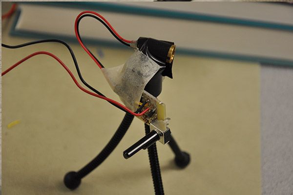
Of course, the user must point the beam at the target and align the reflection with the receiver. The transmitter is simply a laser mounted on a steady post or tripod, with an on/off switch. The receiver must also be steady and adjustable, but includes the majority of the components. The phototransistor is the key to the receiver, and must be aligned well to ensure accurate operation. Laser light is used for its low divergence. Whereas normal light spreads out in three dimensions, laser light travels in a tight cone, so the reflected beam is still strong. Also, laser light is coherent, so the energy is concentrated at a single frequency, making it easier to detect.
The main hardware/software trade-off was deciding which functionality would be implemented in hardware and which in software. Although digital filtering was a possibility, we decided that analog filtering should be sufficient. Also, the signal could be recorded to a computer and post-processing would be more practical from a full computer rather than a microcontroller.
To understand more about FFTs, refer to the section below.
ANSI 136.1 provides laser standards. Relevant lasers are in Class II for less than 1 mW and Class IIIa for less than 5 mW. Based on a blink reflex of 0.25 seconds, Class II lasers are considered safe. With restricted beam view and careful handling, Class IIIa lasers, if altered by optical instruments, may seriously damage the retina if stared at for two minutes. These are typical for laser sights in firearms or laser pointers. We use a laser rated at 4 mW, making it Class IIIa. The safety implications are discussed later. We do not believe that any other standards are relevant to our project.
We did not discover any relevant patents, trademarks, or copyrights. Similar systems have been implemented before, so the base technology is not new, although we have not found any optical microphones involving a microcontroller.
The FFT
In order to output the spectral analysis, a Fast Fourier Transform is performed on the incoming audio signal. For peak microcontroller performance, we only perform the forward FFT using real-valued input. Before we get into more detail about this, we will first discuss the Fourier Transform and its implications.
The Fourier Transform is a transition from the time domain to the frequency domain that can be computed in both continuous and discrete time. As we are using a microcontroller to perform a series of analog to digital conversions, we will talk about the Discrete Fourier Transform, or DFT.
A DFT performs computation on, and outputs, a series of discrete, imaginary numbers. In our case, the set of discrete numbers is the array of regularly-spaced samples from the ADC. The output will have the same number of values as the input, each representing 2*F/N, where F is the highest frequency and N is the number of samples. The reason why it is 2*F/N rather than F/N is because the final output is symmetric. Several different FFTs exist; the one we use is decimation-in-time. This algorithm efficiently performs the DFT, taking advantage of several properties of the DFT. The main advantage is that signals can be split into half, creating two signals. Then, each of these signals can be split in half, into even and odd terms, and so the DFT can be performed on the new signals, as in the equation below (from Professor Delchamps)
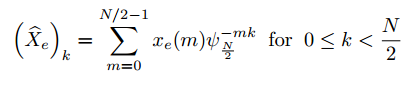
If N is a power of 2, this computation is very efficient due to its recursive nature.
Each output value is referred to as a bin, and under the results section we show the peak frequency represented by each bin in our final representation of the code. In order to calculate the magnitude, or power, of this result we take the sum of squares of the real and imaginary parts.
In order to calculate F, we refer to the Nyquist sampling theorem, which states that it is necessary and sufficient to sample at twice the maximum frequency of the signal. Under the Program Design section, we discuss what sampling frequencies we chose for each mode of operation.
The algorithm for a “classic” DFT has rather high time complexity, and so we use a Fast Fourier Transform adapted from Tom Roberts and Malcolm Slaney by professor Bruce Land of Cornell University. The time complexity of this algorithm is much less, allowing us to take a higher number of samples to improve our accuracy.
This algorithm performs an FFT using 8:8 fixed point arithmetic, again as a speed increase. We expect the values of our ADC to be between -0.5 and 0.5 before performing the FFT, and thus need to handle a certain level precision after the decimal point. Floating point arithmetic is too time intensive, and again to simplify our time complexity this avoids it.
Program Design
Microcontroller and Software
Our program is split into three logical steps: ADC conversion, FFT calculation, and LCD display of the spectral analysis. The results of the ADC are stored in a buffer the size of the number of required samples to perform the FFT. We finalized our implementation with taking 32 samples. It is important to note that we need to format the result of the ADC into fixed point form to be compatible with the fixed point FFT algorithm. Knowing that the results of an ADC conversion are between 0 and 255, we subtract this result by 128 to center it around 0 and store this in the lower 8 bits of an integer.
We have the following ADC sample frequencies for the different modes of operation. For the 500Hz range, we sample every 0.756ms, or 1142.85Hz, for the 1200Hz range, we sample every 0.375ms, or 2666.67Hz, and for the 4000Hz range, we sample every 0.125ms, or 8000Hz. We see that this stays true to the Nyquist theorem (discussed above). Switching between these frequency ranges is completed using a single button in a 3 state state-machine. At each button press we move from 500Hz -> 1200Hz -> 4000Hz then back to 500Hz. The press of a button triggers an interrupt which handles this state transition. Additionally, we have 3 LEDs one of which is illuminated in each state to notify the user what frequency range they’re in.
Once we have 32 ADC samples in fixed point format, we’re ready to run the fixed point FFT algorithm*. Running the FFT algorithm performs the math listed above, and returns a real and imaginary array both the size of the number of samples (32). The last step in the FFT process is to calculate the magnitude of the result by summing the square of the real and imaginary parts. This produces the power and allows us to perform a spectrum analysis.
In order to display the spectral analysis, we first needed to make a new library of bars to output to an LCD using lcd_lib**. To do this we defined 9 different bars (ranging from size 0 to size 8). We then wrote a function that takes a series of 16 inputs ranging from 0 to 16 and outputs the correct 16 bars using the 32 characters on our LCD display. It does this by putting the necessary two bars on top of each-other to create “two-level bars.” For example if a bar is intended to be size 13, it is represented by a bar of size 5 on top of a bar of size 8. Once we receive our magnitude from the FFT algorithm, we need to scale the result into 16 uint8_t’s ranging from 0-16. In order to improve the performance of our system, we only update a character if it is different than it was in a previous timestep.
We decided to remove the symmetry from our system by only displaying the first 16 bins of our 32 results from running FFTfix. We made this choice to maximize our usage of the LCD display as it is only 16 characters wide, and outputting the symmetric result limits the precision of each bin.
Our main function performs these 4 routines in an infinite while loop: ADC sample, FFTfix, FFTmag, and draw_fft. As soon as one is done, we immediately move to the other.
In the source code (at the end), we explain in comments each method that we used in our final program.
* The fixed point FFT algorithm is from Professor Bruce Land which was adapted from code by Tom Roberts (11/8/89) and Malcolm Slaney (12/15/94)
** lcd_lib is from scienceprog.com (2007), made available to us through Professor Bruce Land
Hardware Design
This system has very direct relationships between the analog parts and the digital parts. The analog hardware acquires and prepares the signal to be sent to the microcontroller, but the digital side doesn’t control the analog circuitry beyond indicator LEDs and the LCD.
The hardware was designed to perform the overall goal of implementing an optical microphone using several stages. The first stage supplies the correct current to the laser transmitter to produce a sufficiently bright beam. The next and most complex stage acquires the reflected beam, amplifies it, and filters out noise. Next, the cleaner signal is sent to two different stages. One amplifies the audio signal for headphones, and the other amplifies the signal to prepare it for analog-to-digital conversion in the microcontroller. This latter signal is analyzed by the MCU for frequency content, as described in the previous section, and the resulting spectrum is displayed on the LCD by sending characters from data output pins. Also, the frequency range can be switched between three presets using an input button, and LED indicators show the current state.
Laser transmitter
The laser transmitter simply emits a beam which can be pointed at reflective, vibrating surfaces. The desired functionality includes compatibility with available phototransistors, sufficient and adjustable brightness, and long range. The laser module we selected has a wavelength of 650 nm (red) and less than 2 mrad beam divergence, meaning that it is practical for long ranges (so after 100 ft it grows 5 inches). Using the simple circuit shown in the diagram, a potentiometer controls the brightness of the laser, from dim to very bright. The resistance values were found empirically – with the knob turned all the way down, the 120 ohm resistance gives a bright beam, drawing around 30 mW total. With the knob up all the way, the 120+620 ohm resistance gives a dim yet visible red spot and draws around 10 mW. This works with a typical 9-volt battery. The laser is mounted to a small tripod to aid in alignment.
Receiver and Amplifier
The signal amplifier circuit was designed to handle a weak and noisy signal. The reflected beam spot must be aligned to hit the phototransistor to generate the current which creates the audio signal. The phototransistor chosen has a peak wavelength sensitivity at 800 nm, but at 650 nm, which the laser emits, the sensitivity is 70%. This is more than adequate sensitivity, and using infrared light near 800 nm would be much more difficult to align. Using green light near 500 nm, the sensitivity would only be 10%, and other phototransistors have very similar sensitivity profiles. Additionally, the rise and fall times are 4 microseconds according to the datasheet, so it is more than fast enough to handle audio signals, which are closer to the order of 1 ms.The phototransistor is arranged in a common emitter topology, which was found to work well. The 2 kohm resistor was found to provide acceptable results compared other nominal values tested.

After the common emitter stage, a decoupling capacitor separates the DC bias of the signal from that of the next stage. The capacitor is also part of a high-pass filter, together with the 11k resistor, with a cutoff frequency of 145 Hz (1/2*pi*RC). The ideal pass-band of this stage is 100 Hz – 1 kHz, because human voice can range as wide as 60-7000 Hz, but generally up to only 300 Hz. The cutoff is so high to combat 60 Hz and 120 Hz noise, which can be very strong in a room filled with dozens of computers, equipment and fluorescent lights (not to mention sleepy engineers). The LF353 chip contains two operational amplifiers, both of which involve a low-pass and high-pass part (together band-pass) and gain. This overall topology is based on a common design used in many 4760 projects in the past. The low-pass filter involves the 2.2 nF capacitor and the 100 k resistor, with a 724 Hz cutoff. This pass-band of 145 – 724 Hz removes the DC bias, much of the 60 Hz noise and high frequency noise. The gain is controlled by the ratio of the 100k resistor to the 5.1 k, so it is 20 for each of the two stages. However, the volume potentiometer controls this gain, and so it can adjust the audio output from silence to extreme loudness. Because this system uses a 9-V battery, there are no negative rails available for the op-amps. Instead, the rails of 0 V and 9 V are used, but the input terminals are connected, through resistors, to a separate voltage level of approximately 2.83 V. This level is maintained using several diodes in series. The 8.2k resistor ensures that about 1 mA is going through the diodes, stabilizing the voltage. And thus this stage acquires the audio signal from the reflected beam, amplifies it, removes noise, and isolates the phototransistor from the next stage. (source: http://en.wikipedia.org/wiki/Human_voice)
Parts List:
| Part | Price | Quantity | Total Price |
|---|---|---|---|
| Custom PC Board | $4 | 1 | $4 |
| 9-Volt battery | $2 | 1 | $2 |
| Mega1284 | $5 | 1 | $5 |
| LCD | $8 | 1 | $8 |
| Mini Tripod | $1.89 | 1 | $1.89 |
| Solder Board | $2.50 | 2 | $5 |
| Phototransistor | $0.56 | 1 | $0.56 |
| White board | $6 | 1 | $6* |
| Jumper Wires | $1 | 10 | $10* |
| Red Laser | From lab | $0 | |
| Resistors | From lab | $0 | |
| Capacitors | From lab | $0 | |
| Op-amps | From lab | $0 | |
| Pushbutton | From lab | $0 | |
| LEDs | From lab | $0 | |
| Wires | From lab | $0 | |
| Flux Capacitor | From lab | $0 | |
| Apple box | Priceless | $0 | |
| *used for demo, but not needed for final design | Total Price | $42.45 |
For more detail: Optical microphone and spectrum analyzer Using Atmega644
- How does the optical microphone acquire sound?
It measures vibrations by detecting changes in a laser beam reflected from a target with a phototransistor, then amplifies and filters the resulting signal. - Can the system display frequency content in real time?
Yes, a microcontroller performs a fixed-point FFT and displays a real-time spectrum on an LCD. - What sampling ranges are available?
Three ranges: 500 Hz (sampling ~1142.85 Hz), 1200 Hz (sampling ~2666.67 Hz), and 4000 Hz (sampling 8000 Hz). - Does the system provide audio output for listening?
Yes, there is an audio amplification stage with a headphone output for monitoring the signal. - How is the laser transmitter powered and adjusted?
The laser is powered from a 9 V battery with a potentiometer controlling brightness and mounted on a tripod for alignment. - What filtering does the analog front end use?
The receiver uses a band-pass topology with a high-pass cutoff ~145 Hz and a low-pass cutoff ~724 Hz to target roughly 145–724 Hz. - How is the FFT implemented on the microcontroller?
It uses an 8:8 fixed-point decimation-in-time FFT adapted from academic code, operating on 32 samples to produce 32 bins and magnitude calculations. - Can the frequency range be changed by the user?
Yes, a single button cycles between the three preset ranges, and LEDs indicate the current state. - Is the phototransistor suitable for the red laser used?
Yes; the phototransistor peak is near 800 nm but has about 70% sensitivity at 650 nm, which is adequate. - What safety class is the laser used?
The laser is rated about 4 mW and classified as Class IIIa; safety implications are discussed in the article.