Summary of Speech Lock
Summary: We implemented a speaker-recognition voice-activated lock on an ATmega1284p using a microphone with hardware filtering and fixed-point DSP. The system extracts Mel-cepstral features via framing, Hamming windowing, FFT, Mel filterbank weighting, log, and DCT, then uses Linde-Buzo-Gray vector quantization for training and Euclidean-distance matching for testing. It runs in real time, provides LCD feedback, and stores up to three trained centroid sets. Accuracy is demonstrative but not production-grade.
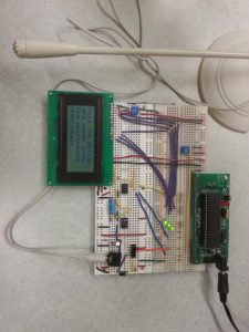
Parts used in the Speech Lock:
- Microphone and preamplifier circuit with low-pass filter
- Analog comparator (for voice activity detection)
- ATmega1284p microcontroller
- ADC (on ATmega1284p)
- LCD display
- User pushbutton (start sampling)
- C firmware implementing FFT, DCT, and VQ (Linde-Buzo-Gray)
- Hamming window coefficient table (C array)
- Mel filterbank coefficient arrays (C arrays)
- UART interface (for debugging)
- Power supply and supporting passive components
we designed and implemented a speaker recognition device that acts as a lock triggered by the sound of your voice saying a specific passcode. The implementation uses hardware filtering from a microphone and many signal processing concepts in software. All software and matching is implemented in the ATmega1284p. The lock has two modes: training and testing. Training mode allows the lock owner to provide voice samples to set the lock, and testing mode is the standard setting in which several users attempt to unlock the lock.
The accuracy of the device is not quite appropriate for a real security system but succeeds in demonstrating functionality. The device executes in real time despite the mathematical complexity underlying the software design and provides the user with feedback on an LCD screen. Results are displayed as value distances from the original speaker’s voice sample, which are compared to a threshold to determine whether the lock is released.
High Level Design
Logical Structure
At a high abstraction our project takes in input speech, extract key features, and compare it to pre-registered signals. We then plan to be able to determine whether or not the speaker is a match with the stored speaker based on their specific speaking features. We use digital signal processing tools to extract speech features, identify common patterns per person, validate patterns based on pre-registered or machine-learned values, and then accept or reject these individuals as the input based on errors calculated in each pattern.
Rationale and Inspiration
We decided to implement this idea because the members of our group enjoy the signal processing aspect of ECE and we were able to find good online sources for a project like this. These sources used MATLab to implement the code and we thought that implementing it on an 8-bit microcontroller with only 8kB of memory would be a good final project.
Background Math
The method we used to determine the relative distance to the preset speaker was Mel cepstrum analysis. This is done using several steps:
- Take the input audio signal and divide it up into multiple frames
- For each frame, find the power spectral density
- Apply the Mel filterbank to the power spectrum
- Normalize the spectral data
- Take the DCT of the filter banks
These steps are all done to closely approximate human hearing to get the best results. The reason we frame the audio signal is to get a relatively unchanging audio signal. We want the input to be simple enough to analyze while long enough to get reliable data from. Dividing up the audio signal into 20-40 millisecond frames will get the best results. The number of samples per frame will obviously depend on sampling rate. Frames can overlap with one another but this is not necessary.
After framing the input signal, we apply a Hamming window to each frame. This window brings the ends of the signal to 0 to minimize ringing and discontinuity. This step is not strictly necessary but provides slightly better results when input signals overlap.
Once we have the frames, we need to analyze their power spectrum. This is most easily and commonly done by taking the Discrete Fourier Transform (DFT) of the frames. The power spectrum also gets the frequency content of the signal which, for audio signals, is much more easily analyzed than the original time domain signal. The DFT is taken by putting each frame into the following equation:
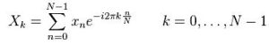
We will only need to keep the first N/2 + 1 coefficients since the highest frequency content is contained in the middle of the FFT coefficients. The positive frequencies are in the lower indices and the negative frequencies are contained in the higher indices.
Once we have the spectral data from the DFT, we need to analyze it. The best way of doing this and getting speaker information is to mimic the human ear as closely as possible. The first step in this analysis is to section off the power at different frequencies. Because the human ear can differentiate frequencies much more closely at lower frequencies (e.g. we can differentiate 620 Hz and 600 Hz much more easily than 2020 Hz and 2000 Hz), we use a logarithmically spaced filterbank to section of these frequencies. The most commonly used filterbank is the Mel filterbank, which we also implemented. The formula for calculating Mels given frequency (in Hertz) is given as follows:
![]()
To separate the power densities into bins, we use triangular filter banks. To find the start and end frequencies, we convert the beginning and end frequencies (in our case, 200 and 4000 Hz) to Mels. We then decide how many bins we want (32) and find that many linearly spaced Mels between our beginning and end frequencies, excluding the two endpoints. Once we have these Mels, we convert them back into frequencies in order to parse. Each frequency will go into 2 bins using this method.
Since we have frequencies in terms of FFT coefficients, we need to figure out a way to get each frequency into the corresponding bin. Converting frequencies to coefficients can be done by plugging in the frequency into the following formula:
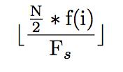
Where N is the number of DFT coefficients, f(i) is the corresponding frequency we are trying to find, and Fs is the sampling frequency.
Now that we have the spectral data sectioned off into bins, we need to take the logarithm of each of these powers to again better imitate the human ear, which doesn’t hear volume on a linear scale. It also lets us use subtraction as a means of finding differences in power, rather than division.
The final step is getting the data we need from the audio input it to take the Discrete Cosine Transform (DCT) of the logarithm Mel cepstral data. This is done to decorrelate the signal since the filter banks overlap. The DCT is done by putting the log filterbank powers into the following:
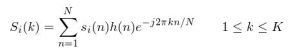
Now we have a set of 32 coefficients for each frame, we throw away the latter half of them, which correspond to the high frequency data and help much less than the others. Once we have all the coefficients we need, we now need to match the DCT coefficients to pre-loaded voice samples.
The method we used to obtain the distances to the recorded voice samples is Vector Quantization (VQ). The first step in VQ is to find the initial centroid of the input space, effectively the average. This centroid is then updated into 2 new centroids by offsetting in every dimension by a small number. For our design, we used ±0.0625. Once we have the offset, we find the Euclidean distance from each of our coefficient vectors to each of the two new centroids. Whichever one is closer, we assign that vector to that centroid. i.e., we assign each vector to the centroid cj that satisfies the equation:
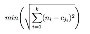
Once this step is done, we simply recursively apply this algorithm to each of the new centroids until we have the number of centroids we want.
Hardware/Software Tradeoffs
The choice between hardware or software implementation came down mostly to what we wanted to use for DSP techniques. Most of the audio filtering we used was much more easily implemented in hardware as it not only gave a more accurate reading, but also it was done with components that were readily available to us. On the other hand, the transform equations we used were easier to do in software as they involved arithmetic and were discrete rather than continuous operations.
Standards
Given that our device has relative few human-to-design interaction, there are no immediately notable IEEE Safety standards – given our time and availability to research – that it is required to adhere too. Provided with more time and need to follow these standards – for a stringent more narrowly tailored set of safety factors – we would research IEEE ISO code on human-design interactions.
Existing Patents
Our design was based on existing academic type literature for commonly accepted methods of speech recognition. Many patents exist expanding on these methods, but the general process itself is, to the best of our knowledge, unpatented. It works through a series of widely known mathematical operations such as the FFT, DCT, and vector quantization.
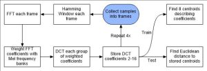
Software Design

The flow chart above describes the process of taking samples all the way to either matching or training the lock. The process begins where the samples are collected into frames.
Almost all values used in software, including the sample values after they are obtained and move through processing, are signed 16-bit fixed point values. These may take on a range from about 128 to -128, with a step size of 1/256.
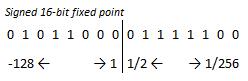
These were chosen over floating point values for mathematical efficiency.
Taking Samples
Since getting voice samples from the microphone circuit involves interfacing with the user, starting the process involves some steps to ease use. We started with only a button that, when pushed, began the cycle of taking in microphone input in the ADC. While we, the creators of the project, had full knowledge of the way this worked, other users tended to press the button and then wait up to a second before speaking. This was a big problem since taking in a second of silence is giant waste of sampling, processing power and storage. To amend this, we set the output of the microphone circuit to go not only to the ADC of the microcontroller, but also to the analog comparator. To start sampling, not only does a button need to be pressed, but the microcontroller must detect that the user is actually speaking.
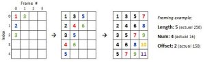
Since the process necessitates placing samples into overlapping frames, for efficiency and memory saving we created an algorithm to save samples directly into frames as they are obtained. The memory efficiency comes from the fact that the same array is used to store the samples as they are scaled and transformed throughout the process flow. It would be an unnecessary waste of space to first store the samples consecutively in a one-dimensional array when they must be must to a frame matrix anyway.
The samples are converted and pulled from the ADC one by one. The ADC is set to 125,000kHz. At 13 cycles of execution, this means the effective sample rate is around 9,600kHz. The cutoff of the low pass filter following the microphone input was measured to be around 3kHz. This satisfies the Nyquist-Shannon sampling condition, which states that to prevent aliasing, sampling must occur at a rate that is at least twice as frequent as the highest frequency rate existing in the signal. The samples from the ADC are shifted left by 6, or multiplied by 64, as a scaling factor. This value was chosen as a trade-off between signal accuracy and ensuring prevention of overflows.
As each sample is obtained from the ADC, it is placed into the frames in each location it belongs. The code does this by taking advantage of the pattern visible in the image above. For instance, you may notice that if a number is to be placed in a given frame at an index greater than or equal to the offset, it must also be placed in the next frame at (index – offset).
Windowing
Following taking the samples into frames, each frame is scaled by the Hamming window.
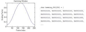
Using MATLAB, we created code to produce a C array with Hamming scaling factors in a fixed point array of length 256. The fixed point values were stored as chars, since they are all less than or equal to one. Each frame of the sample matrix and the hamming array are both looped through and multiplied together, with the outputs overwriting the previous values of the frame matrix.
Fast Fourier Transform
After each frame is multiplied by the Hamming, the FFT is taken. The FFT function used was code created by Tom Roberts and Malcolm Slaney and modified by Bruce Land. The function is fed each frame of the frame matrix individually. The outputs are have both real and imaginary components, which are squared and added together to get the square magnitude of the FFT. This gives us a power spectral density of the input voice samples.
Mel Frequency Band Weighting
The next step is weighting the spectral density with the Mel frequency banks. Similarly to the Hamming window, we used MATLAB to produce C arrays to use for the banks.
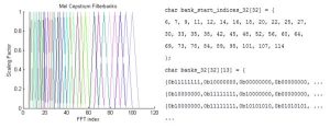
The banks stretch to near the halfway point of the FFT since this is where the highest frequency lies. The banks do not quite reach because of adjustments made to ignore the highest frequencies taken from sampling.
The MATLAB code produces an array and a matrix. The array contains the index at which each Mel bank weighting values begin, and the matrix contains the weighting values themselves all starting at index 0. The purpose of creating a separate array to indicate the start indices of each bank instead of starting the banks at different indices in the matrix is to save memory. Additionally, the values are stored as chars since they are all less than or equal to one.
The weighting is done by looping through each frame, then looping through each bank and saving the coefficients obtained from multiplication indexed from the beginning of the frame matrix. Therefore, after the weighting, only the first 32 values of each frame are of interest.
Discrete Cosine Transform
The DCT is a 32-point DCT of the weighted Mel frequency coefficients. The DCT code was produced by Luciano Volcan Agostini, Ivan Saraiva Silva, and Sergio Bampi and adapted to GCC by Bruce Land. I modified the code slightly to pass in input and output arguments.
From the output of the DCT, coefficients 2 through 16 are kept and added into a separate coefficient matrix. Since there are 16 frames taken by each sample, and 64 coefficient frames are stored total, this entire process repeats 4 times, each time adding more coefficients to the matrix until it is full.
When the matrix storing the 4 sets of coefficients is full, the number of zero-valued coefficients are counted. If the value is larger than a preset value, then a message is displayed on the LCD that a new sample is required. This occurs when too much of the detected input is silence.
Training – Vector Quantization
Vector quantization, as mentioned in the background mathematics section, is a form of data compression used to save information obtained from sample processing for matching later. Vector quantization works as a multi-point mean of the obtained coefficients to produce 8 values representative of the sample data as a whole. Producing a functional vector quantization algorithm in C was one of the most difficult aspects of the project to produce.
We wrote the Linde-Buzo-Gray algorithm for vector quantization, first in MATLAB and then in C to obtain these values. We used MATLAB first as it was much easier to write and debug. The results of the MATLAB code producing 8 centroids from 64 coefficients are shown below.
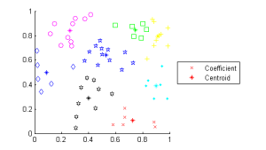
The asterisk marks represent the centroids of each set, and the other shapes represent the coefficients. Each set that is the same color and shape have the same closest centroid, and the centroid position is at the center of the set.
Once the code was written in MATLAB, it was ported to C with some necessary changes for the hardware. Since the algorithm requires division where the denominator cannot be set to a fixed value, it was necessary to use Bruce Land’s divfix algorithm for fixed point division.
It was also necessary to monitor values while looping through the algorithm to ensure no overflows occur throughout the process. To solve the problem of overflows, vector distance values could be shifted as necessary as long as the shifting was consistent to all values. The fact that many parts of the algorithm do not require accuracy of absolute magnitudes but only relative magnitudes was something that could be taken advantage of to improve efficiency. For instance, when it became necessary to find a Euclidean distance from a single point to a centroid and compare it to distances to other centroids, the square root following the sum of squares could be ignored, since the values themselves are not important, only the relative magnitudes of the values.
The UART was crucial to develop and ensure the functionality of the Linde-Buzo-Gray algorithm. The values were compared throughout the process using print statements and comparing the outputs to the functional MATLAB code.
When the function determines the centroid values, they are stored in an array in the system. The MCU is set to store up to three sets of centroids, but can be easily adjusted to store more.
Testing – Euclidean Distance Summing
When testing instead of training, the program takes a different protocol. Looping through each coefficient of the sample set (64 total), the Euclidean distance to each centroid in one of the stored sets of training centroids is determined. The minimum of these distances is added to a running distance counter between the sample and the stored training set.
Source: Speech Lock
- How does the Speech Lock determine a match?
It computes Mel-cepstral coefficients, compresses training data with vector quantization to centroids, then sums minimum Euclidean distances from test coefficients to stored centroids and compares to a threshold. - Can the device run in real time on an ATmega1284p?
Yes, the article states the device executes in real time despite the mathematical complexity. - What feature extraction steps are used?
Framing, Hamming windowing, FFT to get power spectrum, Mel filterbank weighting, logarithm, and DCT to obtain cepstral coefficients. - How many coefficients are retained per frame?
The system computes 32 DCT coefficients per frame and keeps coefficients 2 through 16 for each frame. - How many centroids does vector quantization produce?
The Linde-Buzo-Gray algorithm produces 8 centroids from 64 coefficients for each trained set. - What prevents sampling silence during recording?
The microphone output is routed to an analog comparator so sampling begins only when the MCU detects the user is actually speaking, in addition to pressing the button. - How many training sets can the MCU store?
The MCU is set to store up to three sets of centroids but can be adjusted to store more. - Why were fixed-point values used in software?
Signed 16-bit fixed-point values were chosen over floating point for mathematical efficiency on the microcontroller. - What sampling rate and hardware filter cutoff were used?
The ADC effective sample rate is about 9600 Hz and the low-pass filter cutoff following the microphone was measured near 3 kHz. - Does the system provide user feedback?
Yes, the device provides feedback on an LCD showing distance values and messages when new samples are required.